Discrete Probability Distributions
Introduction to Discrete Probability Distributions in Statistics
Discrete Probability Distributions – Statistics is the heart of data analysis, and one of the most important concepts in statistics is probability distribution. Within this concept, Discrete Distributions play a crucial role when dealing with data that is countable or comes in whole numbers.
In this blog, we’ll walk you through what discrete distributions are, how they work, their types, formulas, how they differ from continuous distributions, and much more.

What Is a Discrete Distribution?
A Discrete Distribution is a statistical distribution that shows the probability of outcomes of a discrete random variable. A discrete random variable is a variable that can only take specific, separate values – usually whole numbers.
- In simpler words, if you can count the outcomes (like the number of students in a class, number of cars in a parking lot, or number of heads in 10 coin flips), it’s a discrete random variable, and the associated probability distribution is a discrete distribution.

How It Works
Here’s how discrete distributions generally work:
- Define the discrete random variable (e.g., number of times a die lands on 6).
- List all possible outcomes (e.g., 0 times, 1 time, up to n times).
- Assign probabilities to each outcome using mathematical formulas or experimental data.
- Make predictions or calculate expected values based on the distribution.
For example, in a coin toss:
- The variable can take two values: 0 (tails) or 1 (heads).
- The probability distribution assigns a 0.5 chance to each outcome.
Types of Discrete Distributions
There are several types of discrete distributions in statistics. Here are the most common and important ones:
1. Binomial Distribution
2. Poisson Distribution
3. Geometric Distribution
4. Hypergeometric Distribution
5. Negative Binomial Distribution
1. Binomial Distribution
This distribution is used when there are only two possible outcomes (success or failure), and you are conducting multiple independent trials.
Example: Tossing a coin 10 times and counting how many heads appear.
Formula:
P(X=k) = \begin{pmatrix}n \\k \end{pmatrix}p^{k}(1-p)^{n-k}
Where:
- n = number of trials
- k = number of successes
- p = probability of success
2. Poisson Distribution
Poisson distribution is used to model the number of times an event occurs in a fixed interval of time or space, given that these events occur with a known constant mean rate and independently of the time since the last event.
- Example: Number of emails received in an hour.
Formula:
P(X=k) = \frac{e^{-lambda}lambda^{k}}{k!}
Where:
- lambda(λ) = average rate of success
- k = actual number of events
- e ≈ 2.71828
3. Geometric Distribution
This models the number of trials needed to get the first success in a series of independent Bernoulli trials.
- Example: Flipping a coin until you get heads.
Formula:
P(X=k) = (1-p)^{k-1} p
Where:
- p = probability of success
- k = trial number on which first success occur
4. Hypergeometric Distribution
Used when sampling without replacement. It shows the probability of a certain number of successes in a fixed number of draws from a finite population.
- Example: Drawing 3 red balls from a bag containing 5 red and 5 blue balls.
5. Negative Binomial Distribution
This is a generalization of geometric distribution. It calculates the probability that the k-th success occurs on the n-th trial.
- Example: Number of basketball shots needed to make 3 successful baskets.
How to Calculate Discrete Probability Distribution
Here’s a step-by-step method to calculate a discrete probability distribution:
- Step 1: Identify All Possible Outcomes
List all the possible outcomes of the random variable. - Step 2: Determine the Probabilities
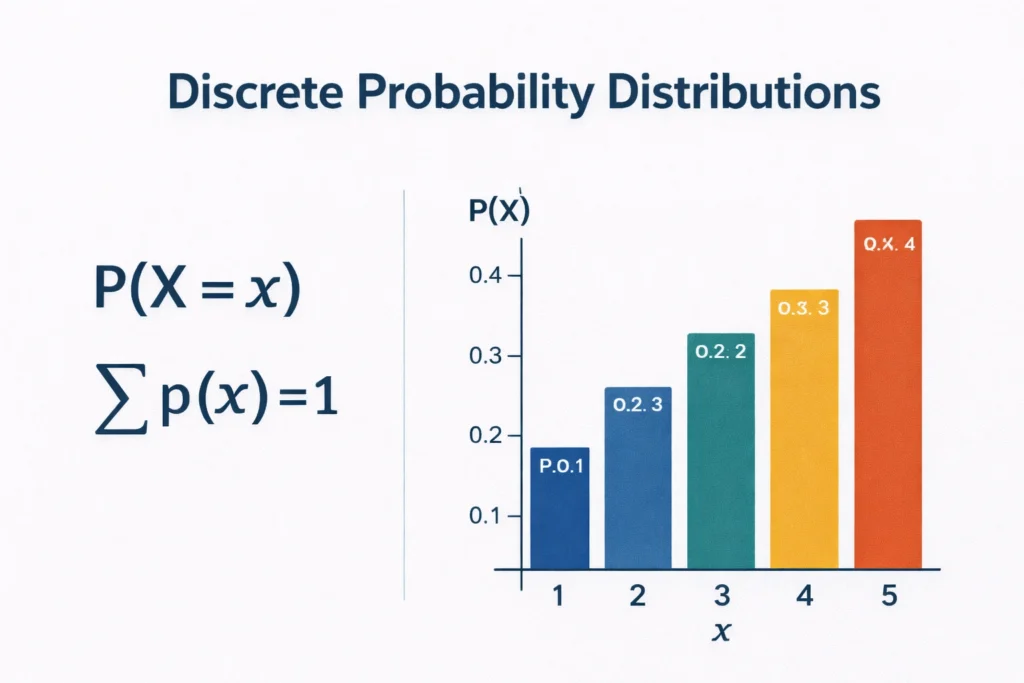
Use logical reasoning, experiments, or formulas to assign probabilities. - Step 3: Ensure the Sum Equals 1
Verify that the total sum of all probabilities equals 1.
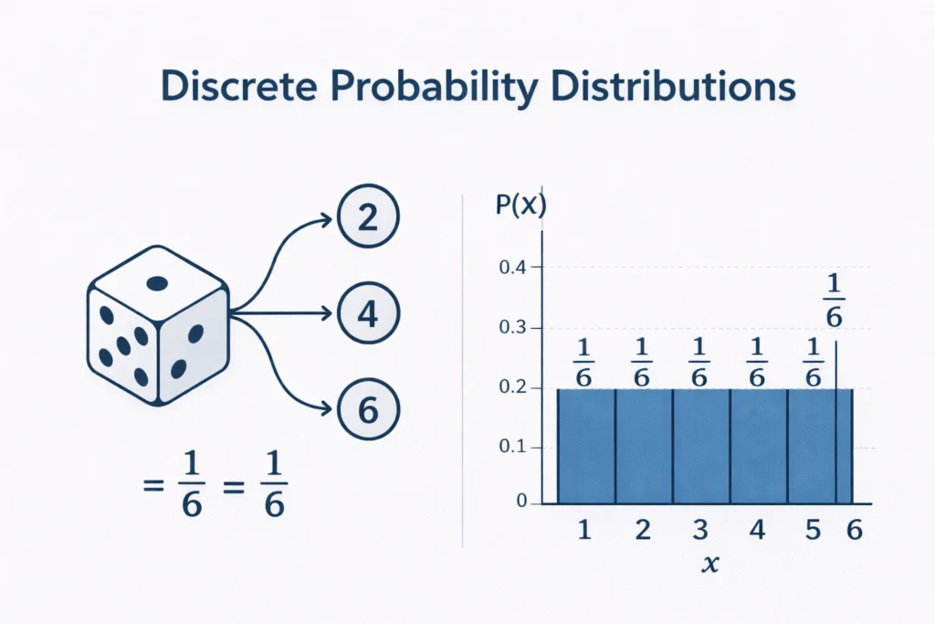
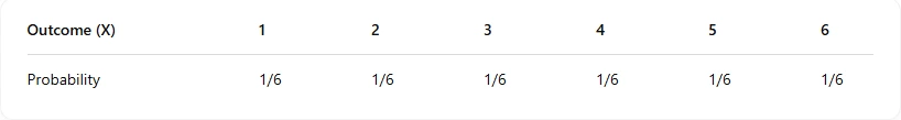
Example: Tossing a Fair Die
Let X be the random variable representing the result of a die roll.
Here, all outcomes are equally likely, and the total probability is:
1/6+1/6+1/6+1/6+1/6+1/6 = 1

Discrete vs. Continuous Distributions
Feature | Discrete Distribution | Continuous Distribution |
---|---|---|
Type of Variable | Countable (e.g., 0, 1, 2…) | Measurable (e.g., 1.5, 2.3…) |
Probability | Assigned to specific values | Assigned over a range |
Examples | Number of students | Height of students |
Graph Type | Bar graph | Curve (PDF – Probability Density Function) |
Probability Formula | P(X = x) | P(a < X < b) |
Real-Life Applications of Discrete Distributions
- Manufacturing: Defective products count
- Healthcare: Number of patients visiting a clinic
- Retail: Number of items sold in a day
- Finance: Number of defaults on loans
- Telecommunications: Call arrivals at a call center
Important Characteristics of Discrete Distributions
- Probability Mass Function (PMF): Defines the probability of each outcome.
- Expected Value (Mean): The average outcome over many trials.
- Variance: Measures the spread of the distribution.
- Skewness: Tells if the distribution leans left or right.
The Bottom Line
Understanding discrete distributions is key to interpreting data where outcomes are countable. Whether it’s flipping a coin, rolling a die, or calculating the number of customer arrivals, discrete distributions give you the tools to make accurate predictions and data-driven decisions.
- From binomial to hypergeometric, each type of discrete distribution has its unique use-case, formula, and significance.
- If you master the concepts of probability, outcomes, and their calculations, you’ll have a strong foundation for further study in data science, machine learning, and statistical analysis.
To Wrap it Up
To wrap it up, a discrete distribution helps you understand the probability of countable events. It’s widely used in many industries, from business to healthcare. Each type – binomial, Poisson, geometric, etc. – has its own use and formula.
Always remember:
- Probabilities must sum to 1.
- Outcomes are distinct and countable.
- Useful for modeling real-world scenarios with exact values.
FAQ's
Discrete distributions deal with countable outcomes (like 1, 2, 3), while continuous distributions deal with measurable outcomes (like 2.5, 3.14).
No, a distribution can either be discrete or continuous, depending on the type of data the random variable represents.
Age is considered a continuous variable because it can be measured in fractions (like 23.5 years), even though we often round it to whole numbers.
You should use the Poisson distribution since it models the number of occurrences in a fixed interval.