
Continuous Probability Distributions
Introduction to Continuous Probability Distributions
Continuous Probability Distributions – In the world of statistics, we often deal with data that can take on a range of values. When these values are not limited to specific numbers but can fall anywhere within a range, we call them continuous.
A continuous distribution describes the probabilities of the possible values of a continuous random variable. These distributions are essential in modeling real-world phenomena like height, weight, temperature, or time.
For example, the height of students in a class could be 160.1 cm, 160.15 cm, or even 160.157 cm. There is no gap between values, making it continuous.

Probability Density Function (PDF)
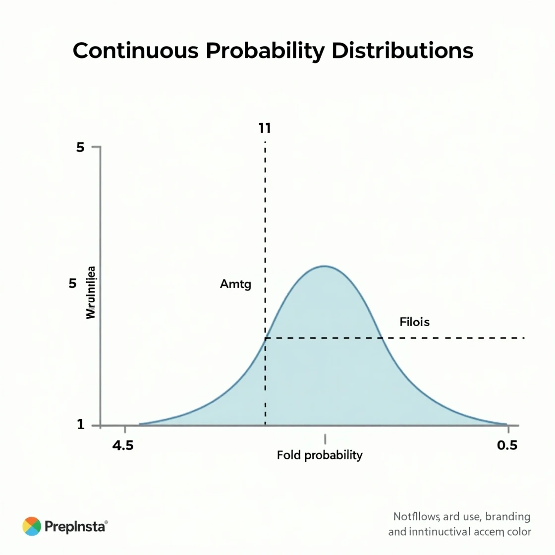
The Probability Density Function (PDF) is a function that describes the likelihood of a continuous random variable taking on a particular value. However, unlike discrete distributions, the probability that a continuous variable is exactly equal to a specific value is zero.
- Instead, the PDF tells us the relative likelihood that the variable falls within a particular range.
- The area under the curve of the PDF between two values represents the probability that the variable lies in that range.
PDF is used to calculate probabilities over intervals.
Example of Continuous Probability Distributions:
For a normal distribution, the PDF curve is bell-shaped. The probability that a value lies between two points can be calculated using this curve.


Cumulative Distribution Function (CDF)
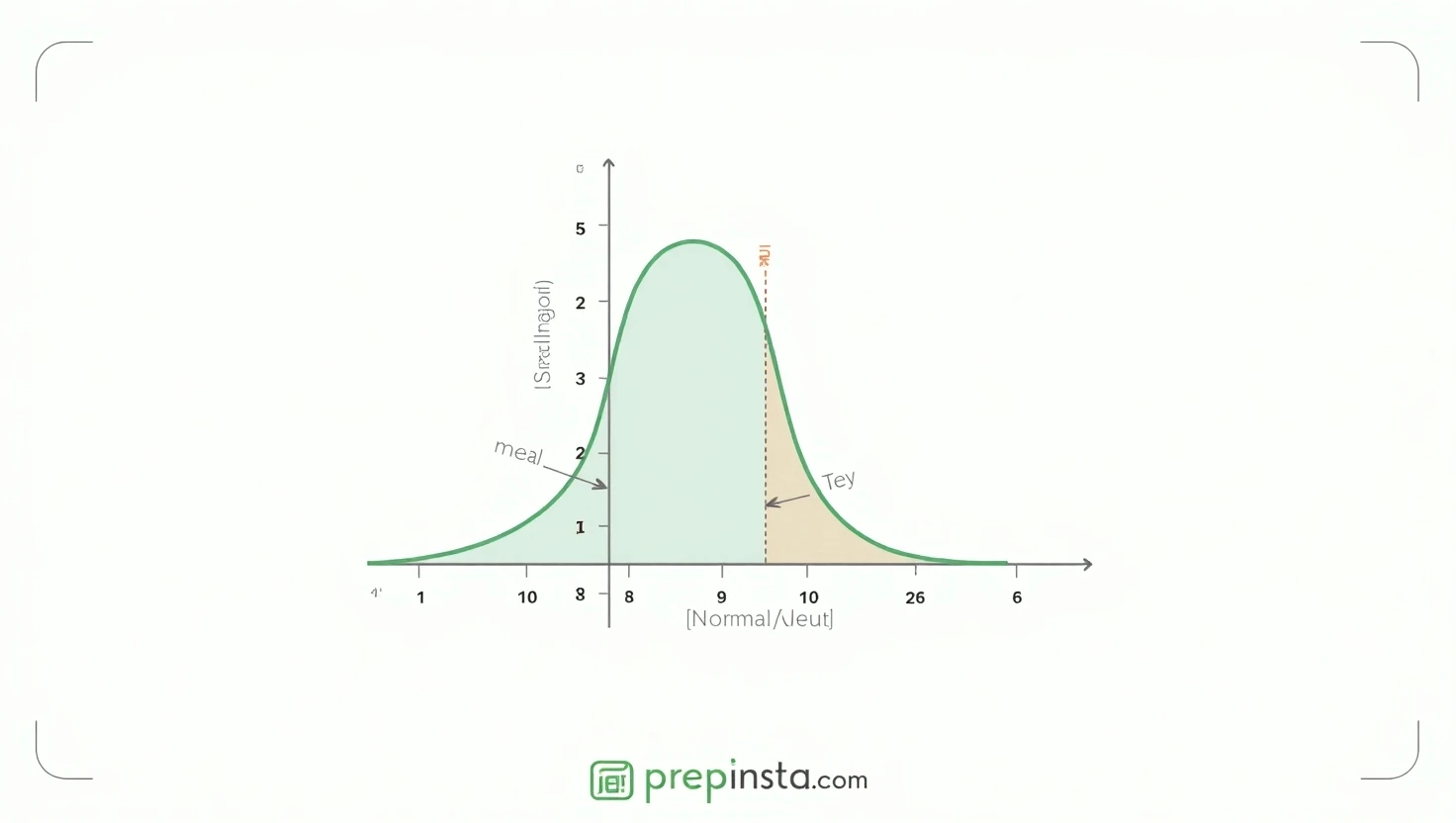
The Cumulative Distribution Function (CDF) gives the probability that a random variable is less than or equal to a certain value. It is obtained by integrating the PDF from −∞ to a specific value.
Mathematically, for a random variable X:
CDF(x) = P(X ≤ x)
Key Points:
- CDF increases from 0 to 1.
- It gives the accumulated probability up to a point.
If you’re looking at a temperature reading, the CDF tells you the probability that the temperature will be less than or equal to a particular value.
Characteristics of Continuous Distributions
- Infinite Possibilities: Values can be any number within a range.
- Probability Density: Probabilities are given over intervals, not at exact points.
- Area Under the Curve: Represents the probability over an interval.
- Mathematical Functions: Described by PDFs and CDFs.
- Smooth Graphs: The graph of a continuous distribution is usually a smooth curve.
Common Types of Continuous Distributions
Here are some widely used continuous distributions:
- Normal Distribution:
- Bell-shaped and symmetric.
- Mean, median, and mode are equal.
- Many natural phenomena follow this distribution.
2. Uniform Distribution:
- All outcomes are equally likely.
- PDF is flat between two points.
3. Exponential Distribution:
- Models the time between events in a Poisson process.
- Common in survival analysis and reliability engineering.
4. Beta Distribution:
- Used in Bayesian statistics and project modeling.
5. Gamma Distribution:
- Generalization of the exponential distribution.
6. Log-normal Distribution:
- Used when the logarithm of the variable is normally distributed.
Applications of Continuous Distributions
Continuous distributions are used across various fields:
- Healthcare: Modeling blood pressure, body temperature, and cholesterol levels.
- Engineering: Reliability and failure time analysis.
- Economics: Modeling income distribution, inflation rates.
- Weather Forecasting: Predicting temperature and rainfall.
- Machine Learning: Understanding distributions of input variables.
Comparison: Continuous vs. Discrete Distributions
| Feature | Discrete Distribution | Continuous Distribution |
|---|---|---|
| Type of Variable | Countable (e.g., 0, 1, 2…) | Measurable (e.g., 1.5, 2.3…) |
| Probability | Assigned to specific values | Assigned over a range |
| Examples | Number of students | Height of students |
| Graph Type | Bar graph | Curve (PDF – Probability Density Function) |
| Probability Formula | P(X = x) | P(a < X < b) |
Advanced Topics
- Multivariate Continuous Distributions: Involves more than one continuous variable.
- Transformation of Variables: Changing one variable to another while preserving probabilities.
- Parameter Estimation: Using sample data to estimate the parameters (mean, standard deviation, etc.) of a distribution.
- Maximum Likelihood Estimation (MLE): A method to find the parameter values that make the observed data most likely.
Visualization
Visualizing continuous distributions helps understand their behavior:
- Histogram: Useful for visualizing sample data.
- PDF Curve: Shows the shape of the distribution.
- CDF Curve: Shows cumulative probability.
For example, a bell-shaped curve in a normal distribution helps identify where most data points lie (within one standard deviation).
To Wrap it Up
Continuous distributions play a crucial role in statistics and data analysis. From natural sciences to finance and artificial intelligence, these distributions help in modeling and understanding complex real-world scenarios.
By learning about PDFs, CDFs, and the types of continuous distributions, we grab ourselves with tools to make decisions. Visualization and proper calculations make it even easier to interpret and apply these concepts in different kinds of problems.
Frequently Asked Questions
Answer:
A continuous probability distribution is a type of probability distribution where a random variable can take any value within a given range. Unlike discrete distributions, continuous distributions are measured over intervals rather than specific values. Common examples include the normal distribution, exponential distribution, and uniform distribution.
Answer:
The main difference is that discrete probability distributions deal with countable values (like number of students), while continuous probability distributions deal with measurable values (like height, weight, or time). Continuous distributions use probability density functions (PDF) instead of probability mass functions (PMF).
Answer:
A Probability Density Function (PDF) is a function that describes the likelihood of a continuous random variable falling within a particular range of values. The total area under the PDF curve is always equal to 1, which represents total probability.
Answer:
Some widely used continuous probability distributions in statistics and data analytics include:
- Normal Distribution (Gaussian Distribution)
- Uniform Distribution
- Exponential Distribution
- Beta Distribution
- Gamma Distribution
These distributions are commonly used in data science, machine learning, and statistical analysis.
Answer:
Continuous probability distributions help analysts model uncertainty, analyze trends, and make predictions based on real-world data. They are important in data analytics for tasks like risk analysis, forecasting, statistical modeling, and quality control.
Answer:
The Cumulative Distribution Function (CDF) shows the probability that a random variable is less than or equal to a certain value. It is calculated as the area under the probability density function curve up to a specific point.