
Running Time Analysis

Running Time Analysis
Running Time Analysis Is a Process of determining how processing time of a problem increase as the size of the problem (Input Size) increases. It’s worth noting that an algorithm’s performance may vary when applied to diverse input types.
As the input size expands, this performance is subject to alteration. Here on this page we will go deep inside of Asymptotic notations.
- It helps determine which algorithm is faster, especially for large inputs.
- Running time is expressed using Big O notation like O(1), O(n), O(log n), O(n²), etc.
What is Running Time Analysis ?
It is the process of determining how processing time of a problem increases as the size of the problem (input size) increases. Input size is the number of elements in the input, and depending on the problem type, the input may be of different types.
Example:
- Size of an array
- Polynomial degree
- Number of elements in matrix
- Number of bits in the binary representation of the input
- Vertices and edges in the graph
How to Compare Algorithms?
To compare algorithms, let us define a few objective measures
- Execution Times? Not a good measure as execution time are specific to a particular computer
- Number of statements executed? Not a good measure as the number of statements varies with programming languages as well as with the style of individual programmer
- Ideal Solution? Let us assume that we express the running time of a given algorithm as a function of input size n(i.e., f(n)) and compare these different functions corresponding to running times. This kind of comparison is independent of machine time, programming style, etc. We measure the total number of basic operations (additions, subtractions, increments, multiplications, divisions,modulo etc.) performed as a function of input size.

Types of Running Time analysis
To analyse the given algorithm, we need to know with which inputs does the algorithm take less time and with which inputs the algorithm takes a long time.
We have already seen that an algorithm can be represented in the form of an expression. That means we represent the algorithm with multiple expressions:one for the case where it takes less time and another for the case where it takes more time.
Three types of analysis are generally performed:
- Worst-Case Analysis: The worst-case consists of the input for which the algorithm takes the longest time to complete its execution.
- Best Case Analysis: The best case consists of the input for which the algorithm takes the least time to complete its execution.
- Average case: The average case gives an idea about the average running time of the given algorithm.

Prime Course Trailer
Related Banners
Get PrepInsta Prime & get Access to all 200+ courses offered by PrepInsta in One Subscription
Running time analysis of algorithms
Running time analysis, also known as time complexity analysis, is a way to estimate the efficiency of an algorithm in terms of the time it takes to execute as a function of the input size. The goal is to understand how the algorithm’s performance scales with larger inputs.
Running time analysis of algorithms example
| Time Complexity | Name |
|---|---|
| 1 | Constant |
| log n | Logarithmic |
| n | Linear |
| n log n | Linear Logarithmic |
| n^2 | Quadratic |
| n^3 | Cubic |
| 2^n | Exponential |
| n! | Factorial |
Asymptotic Notations For Running Time Analysis
We aim to identify upper and lower bounds by doing worst case, average case and best case
analysis. To represent the upper and lower bounds, we need some kind of syntax, and that is the
subject of the following discussion. Let us assume that the given algorithm is represented in the
form of function f(n).
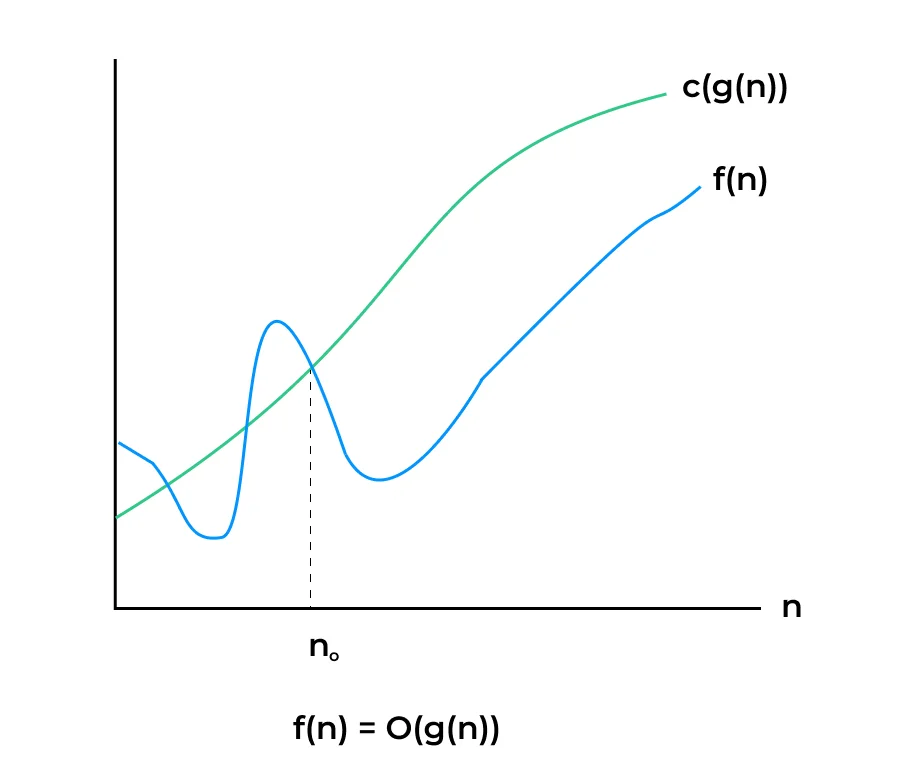
- Big-O Notation:This notation gives the tight upper bound of the given function. Generally, it is represented as f(n)=O(g(n)). That means at larger values of N the upper bound of a f(n) is g(n). For example: if f(n) = n^4 + 2n^3 + 100n + 500 is the given algorithm then n 4 is g(n). That means g(n) gives the maximum rate of growth for f(n) at larger values of n
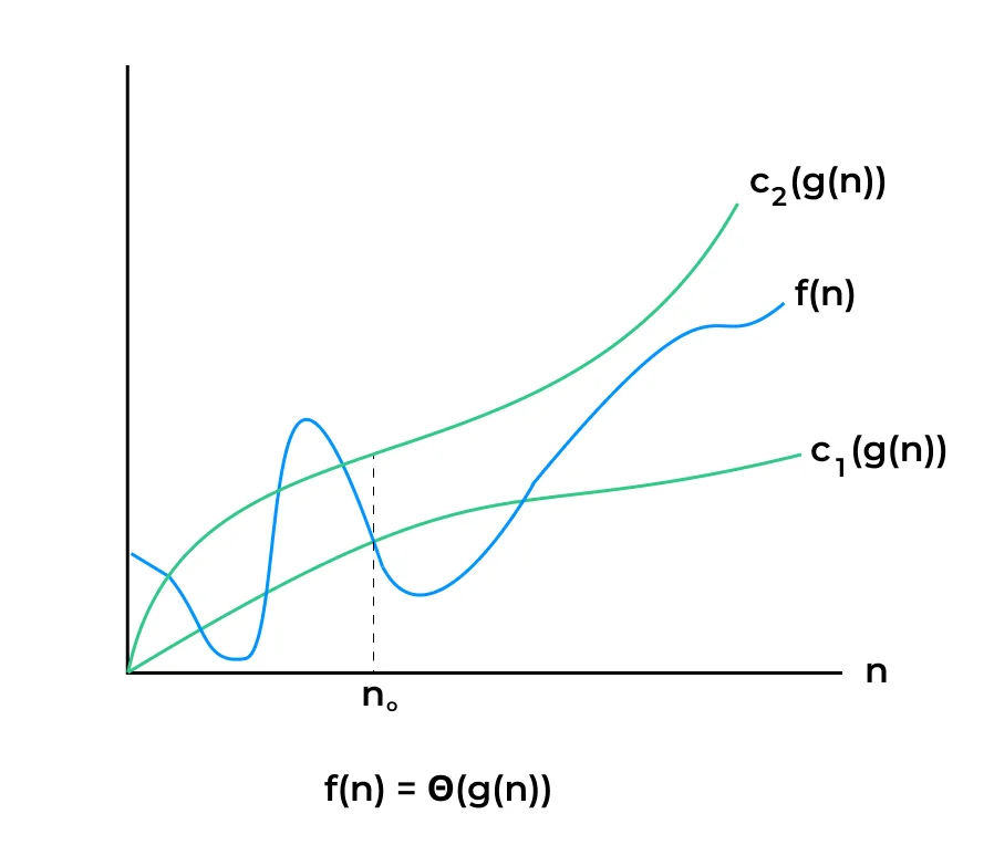
- Big-θ Notation: This notation decides whether the upper and the lower bound of the given function(algorithm) are the same. The average running time of an algorithm is always between the lower bound and the upper bound. If the upper bound(O) and the lower bound(Ω) give the same result, then the Θ notation will also have the same rate of growth. As an example, let us assume that f(n) = 10n+ n is the expression. Then, its tight upper bound g(n) is O(n). The rate of growth in the best case is g(n) = O(n).
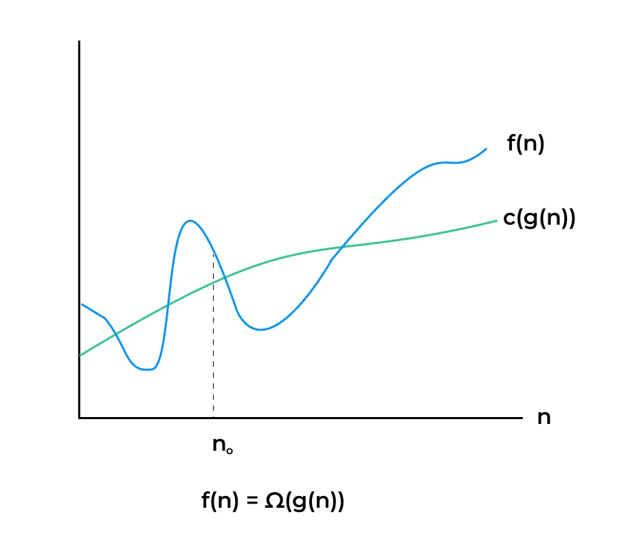
- Big-Ω Notation: Similar to the O discussion, this notation gives the tighter lower bound of the given algorithm and we represent it as f(n) = Ω(g(n)). That means, at larger values of n, the tighter lower bound of f(n) is g(n). For example, if f(n) = 100n2+10n+50, g(n) is Ω(n2).
Example:
import time

def linear_search(arr, target):
    for i in range(len(arr)):
        if arr[i] == target:
            return i
    return -1

# Create a large list of elements
n = 1000000
data = list(range(n))
target = n - 1

# Measure running time
start_time = time.time()
index = linear_search(data, target)
end_time = time.time()

print("Target found at index:", index)
print("Running Time: {:.6f} seconds".format(end_time - start_time))
Output:
Target found at index: 999999
Running Time: 0.072360 seconds
Explanation:
- The function linear_search loops through the list to find the target.
- The larger the list, the more time it takes in the worst case → linear growth.
- Time is calculated using time.time() before and after execution.
- This helps in real-world performance measurement along with theoretical Big-O analysis.
Time and Space Complexity:
| Step | Operation | Time Complexity | Space Complexity |
|---|---|---|---|
| Loop through list | for i in range(len(arr)) | O(n) | O(1) |
| Comparison in loop | if arr[i] == target | O(1) | O(1) |
| Best Case | Target at start | O(1) | O(1) |
| Worst Case | Target at end / not found | O(n) | O(1) |
To Wrap up with:
In conclusion, The key notations—Big O, Omega, Theta, and Little O—each have their unique roles in characterizing algorithmic behavior, whether it’s identifying worst-case scenarios, best-case performance, or providing tight bounds on efficiency. These notations simplify algorithmic analysis, aid in making informed decisions when selecting algorithms, and are essential for evaluating the scalability and performance of software systems.

FAQs
Running time analysis evaluates how the execution time of an algorithm grows with input size. It helps in comparing different algorithms’ efficiency and choosing the most optimal one.
Big-O notation expresses the upper bound of an algorithm’s running time in terms of input size
𝑛
n. It helps estimate the worst-case performance and scalability of algorithms.
Best-case refers to the minimum time taken, average-case is the expected time across inputs, and worst-case shows the maximum time. These help in understanding the behavior of algorithms under different conditions.
By identifying loops, recursive calls, and operations inside them, we calculate how frequently they execute relative to input size
𝑛
n. This gives an estimate like O(n), O(n²), etc., showing time growth.
Get over 200+ course One Subscription
Courses like AI/ML, Cloud Computing, Ethical Hacking, C, C++, Java, Python, DSA (All Languages), Competitive Coding (All Languages), TCS, Infosys, Wipro, Amazon, DBMS, SQL and others