Dijkstra’s algorithm in Python

Dijkstra’s algorithm implementation in Python
Dijkstra’s algorithm, a fundamental concept in computer science, calculates the shortest path between graph nodes. Widely used in navigation, network routing, and resource optimization, it’s essential for solving complex network problems.
In this tutorial, we’ll simplify its logic and Python implementation, equipping you to efficiently apply it to real-world challenges. Let’s dive in!
Purpose and use cases
The primary purpose of Dijkstra’s algorithm is to find the shortest path between two nodes in a graph, particularly in scenarios where finding the most efficient route is essential.

Here are some common use cases and applications of Dijkstra’s algorithm:
- Routing and Navigation: GPS systems, network routing, and public transportation routes.
- Transportation and Logistics: Optimizing delivery routes and public transportation schedules.
- Telecommunications: Efficient communication routes and circuit switching in networks.
- Resource Allocation: Optimizing resource utilization and project scheduling.
- Robotics and AI: Path planning for robots and game character movements.
- Geography and Cartography: Visualizing geographical features and planning exploration routes.
- Wireless Sensor Networks: Efficient data aggregation in sensor networks.
What is a real life example of Dijkstra?
Ans. A real-life example of Dijkstra’s algorithm in action is in GPS navigation systems. When you enter a starting point and a destination in a GPS app, the application uses Dijkstra’s algorithm to calculate the shortest route between these points based on various factors like distance, traffic conditions, and estimated travel time. The algorithm helps the GPS system find the most efficient path for you to reach your destination, guiding you through the roads that will take the least amount of time to travel.
What is Dijkstra’s algorithm with example?
Example :
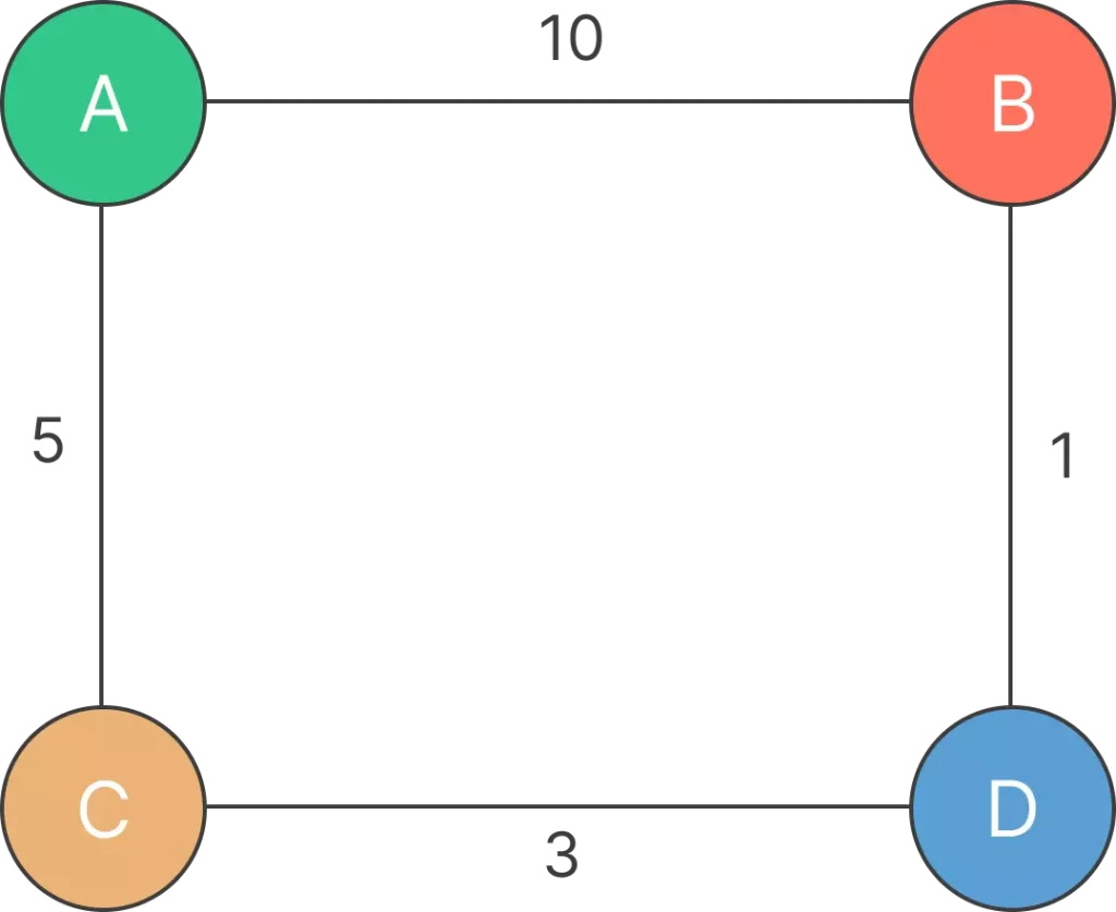
Consider the following graph:

In this graph, nodes A, B, C, and D are connected by edges with the specified weights.
Step 1: Initialization:
- Mark all nodes as unvisited.
- Assign a tentative distance value to every node. Set the initial node’s distance to 0 and all other nodes’ distances to infinity.
- Set the initial node (A) as the current node.
B:

C:

D:

Step 2: Iteration:
- Iteration 1: Consider neighbors of A (B and C).
- For B: The tentative distance from A to B is 0 (current distance to A) + 10 (weight of AB edge) = 10. Update B’s distance.
- For C: The tentative distance from A to C is 0 (current distance to A) + 5 (weight of AC edge) = 5. Update C’s distance.
- Iteration 1: Consider neighbors of A (B and C).
Updated distances: A: 0, B: 10, C: 5, D: ∞
- Iteration 2: Choose the node with the smallest tentative distance (C).
- Consider neighbors of C (A, D).
- For A: The tentative distance from C to A is 5 (current distance to C) + 5 (weight of CA edge) = 10. No update needed for A.
- For D: The tentative distance from C to D is 5 (current distance to C) + 3 (weight of CD edge) = 8. Update D’s distance.
Updated distances: A: 0, B: 10, C: 5, D: 8
- Iteration 3: Choose the node with the smallest tentative distance (D).
- Consider neighbors of D (B).
- For B: The tentative distance from D to B is 8 (current distance to D) + 1 (weight of DB edge) = 9. No update needed for B.
Updated distances: A: 0, B: 9, C: 5, D: 8
Step 3: Termination:
- All nodes have been visited.
Step 4: Path Reconstruction (Optional):
- The shortest paths from A to other nodes can be reconstructed. For example, the shortest path to node B is A -> C -> D -> B with a total weight of 9.
Dijkstra’s algorithm pseudocode:
function Dijkstra(graph, start):
    initialize distances from start to all vertices as INFINITY
    set distance from start to itself as 0
    create a priority queue and add start vertex with distance 0

    while priority queue is not empty:
        current_vertex = vertex with the smallest distance from priority queue
        remove current_vertex from the priority queue

        for neighbor, weight in neighbors of current_vertex in graph:
            calculate potential distance from start to neighbor through current_vertex

            if potential distance is less than current distance to neighbor:
                update distance to neighbor in the priority queue
                update distance from start to neighbor in the distances array
                set current_vertex as the parent of neighbor

    return distances array (shortest distances from start to all vertices)
Implementing Dijkstra’s Algorithm in Python:
Dijkstra’s algorithm:
1. Importing Required Modules:
import heapq
The code imports the heapq module, which provides an implementation of the heap queue (priority queue) algorithm.
2. Dijkstra’s Algorithm Implementation:
def dijkstra(graph, start):
    distances = {node: float('infinity') for node in graph}
    distances[start] = 0
    priority_queue = [(0, start)]
- The dijkstra function takes two parameters: graph (the graph represented as an adjacency dictionary) and start (the starting node for finding shortest paths).
- It initializes a distances dictionary, setting the initial distance to infinity for all nodes except the start node, which is set to 0.
- priority_queue is a list used as a min-heap to keep track of nodes and their distances. Each element in the heap is a tuple containing (distance, node).
3. Dijkstra’s Algorithm Iteration:
    while priority_queue:
        current_distance, current_node = heapq.heappop(priority_queue)

        if current_distance > distances[current_node]:
            continue

        for neighbor, weight in graph[current_node].items():
            distance = current_distance + weight

            if distance < distances[neighbor]:
                distances[neighbor] = distance
                heapq.heappush(priority_queue, (distance, neighbor))
- The algorithm iterates as long as the
priority_queueis not empty. - It pops the node with the smallest distance from the
priority_queue. If the extracted distance is larger than the stored distance for the current node, the loop continues to the next iteration. - For each neighbor of the current node, the algorithm calculates a tentative distance. If this distance is shorter than the previously stored distance for the neighbor, the distances dictionary is updated, and the neighbor is added to the priority queue for further exploration.
return distances
5. Example Graph and Output:
graph = {
    'A': {'B': 10, 'C': 5},
    'B': {'A': 10, 'D': 1},
    'C': {'A': 5, 'D': 3},
    'D': {'B': 1, 'C': 3}
}

start_node = 'A'
shortest_distances = dijkstra(graph, start_node)

print("Shortest distances from node", start_node + ":")
for node, distance in shortest_distances.items():
    print(node + ":", distance)
- The provided graph is represented as an adjacency dictionary.
- The dijkstra function is called with the graph and the start_node (‘A’ in this case).
- The shortest distances from node ‘A’ to all other nodes are calculated and printed.
What is Dijkstra’s algorithm What are its advantages and disadvantages?
Advantages:
- Optimality: Dijkstra’s algorithm guarantees the shortest paths from the source node to all other nodes with non-negative edge weights.
- Versatility: It works for both directed and undirected graphs.
- Precision: It is precise and provides accurate results for finding the shortest paths.
- Applicability: Widely used in various applications, including computer networks, transportation systems, and maps.
Disadvantages:
- Non-Negative Weights: Dijkstra’s algorithm cannot handle graphs with negative edge weights, as it assumes that shorter paths are found by summing shorter edges. Negative weights can cause the algorithm to produce incorrect results.
- Complexity with Large Graphs: The algorithm’s time complexity depends on the data structures used. With a simple array, the time complexity is O(V^2), which can be inefficient for large graphs. With a priority queue, the complexity is O((V + E) * log(V)), making it more efficient but still not optimal for very large graphs.
- Memory Usage: The algorithm may require significant memory usage, especially when dealing with large graphs, due to the need to store distances and vertices.
- No Path Preservation: While it finds the shortest distances, Dijkstra’s algorithm does not preserve information about the actual paths. Additional steps are needed to reconstruct paths if the actual path details are required.
Dijkstra’s Algorithm time and space complexity
Space complexity of Dijkstra’s algorithm is O(V2) where V denotes the number of vertices (or nodes) in the graph.
Time Complexity of Dijkstra’s Algorithm is O ( V 2 ) but with min-priority queue it drops down to O ( V + E l o g V ) .
In closing
Dijkstra’s algorithm remains a cornerstone in shortest path computations, with wide-ranging applications from GPS navigation to network routing. Its logical simplicity and precise results make it an essential tool for developers and engineers alike. Understanding its Python implementation empowers you to tackle real-world pathfinding challenges efficiently.
Despite some limitations like handling negative weights and high memory usage in large graphs, Dijkstra’s algorithm remains highly reliable. With optimization techniques like priority queues, it becomes even more powerful. Mastering it not only strengthens your algorithmic knowledge but also equips you for practical problem solving across industries.
Learn DSA
Prime Course Trailer
Related Banners
Get PrepInsta Prime & get Access to all 200+ courses offered by PrepInsta in One Subscription
FAQs
In the network layer, Dijkstra’s algorithm is used for dynamic routing. It calculates the shortest path from a source node to all other nodes in a computer network, enabling efficient packet forwarding and optimal route selection.
Dijkstra’s algorithm finds the shortest path in a weighted graph, ensuring efficiency in applications like network routing. DFS explores a graph systematically, useful for tasks like traversal and element search, but does not guarantee the shortest path.
Dijkstra’s algorithm is faster than DFS for finding the shortest path in a weighted graph, especially in large graphs. However, DFS has its own applications in graph traversal tasks. The choice depends on the specific problem.

Question 1.
What is Dijkstra’s algorithm in network layer?
In the network layer, Dijkstra’s algorithm is used for dynamic routing. It calculates the shortest path from a source node to all other nodes in a computer network, enabling efficient packet forwarding and optimal route selection.

Question 2.
What is Dijkstra’s algorithm and DFS?
Dijkstra’s algorithm finds the shortest path in a weighted graph, ensuring efficiency in applications like network routing. DFS explores a graph systematically, useful for tasks like traversal and element search, but does not guarantee the shortest path.

Question 3.
Is Dijkstra faster than DFS?
Dijkstra’s algorithm is faster than DFS for finding the shortest path in a weighted graph, especially in large graphs. However, DFS has its own applications in graph traversal tasks. The choice depends on the specific problem.
Get over 200+ course One Subscription
Courses like AI/ML, Cloud Computing, Ethical Hacking, C, C++, Java, Python, DSA (All Languages), Competitive Coding (All Languages), TCS, Infosys, Wipro, Amazon, DBMS, SQL and others


Login/Signup to comment