
Classification In Machine Learning
About Classification in Machine Learning
Classification is a fundamental technique in machine learning, used to predict categories or classes based on input data and uncover patterns between variables.
In this article, we’ll explore different types of classification, their applications across various industries, and the underlying principles behind them. Whether you’re a beginner or looking to enhance your knowledge, this guide will help you understand classification and apply it to solve real world problems.
Read on to explore how classification techniques are revolutionizing data analysis and predictive modeling.

Introduction to Classification in Machine Learning
What is Classification?
- Classification is a type of supervised learning. In supervised learning, a model is trained using data where the correct answers (or labels) are already known.
- The model learns from this data and then makes predictions on new, unseen data.
- For example, consider the task of identifying whether an email is spam or not.
- You can train a classification model using a dataset of emails, where each email is labeled as “spam” or “not spam.”
- After training, the model can classify new emails into one of these categories.
Types of Classification In Machine Learning

- Binary Classification: This is when the model predicts one of two categories. A classic example is identifying whether an email is spam or not spam.
- Multiclass Classification: This is when the model predicts one of three or more categories. For example, classifying fruits into categories such as apple, banana, and orange based on their size, color, and shape.
Difference Between Binary and Multiclass Classification
| Aspects | Binary Classification | Multiclass Classification |
|---|---|---|
| Description | Predicts one of two possible categories. | Predicts one of three or more categories. |
| Example | Classifying emails as “spam” or “not spam.” | Classifying fruits as “apple,” “banana,” or “orange.” |
| Algorithms | Logistic Regression, SVM, Decision Trees, etc. | Decision Trees, Random Forest, Neural Networks, etc. |
| Nature of Output | Single output (either 0 or 1, or two possible labels). | Single output, but with multiple possible labels. |
| Applications | Email filtering, disease detection (e.g., cancer: positive/negative). | Object classification (e.g., image recognition with multiple categories). |
Key Concepts in Classification Before diving into algorithms, it's essential to understand some key concepts related to classification:
Training and Testing Data
The data used to build a classification model is typically divided into two sets:
1. Training Data:
- This is the data used to teach the model. It includes both the features and their corresponding labels.
- The model learns from this data to understand the patterns that link the features to the labels.
2. Testing Data:
- This data is used to evaluate how well the model performs on new, unseen data.
- It helps us determine whether the model can generalize well to data it has not seen during training.
Working of Classification In Machine Learning


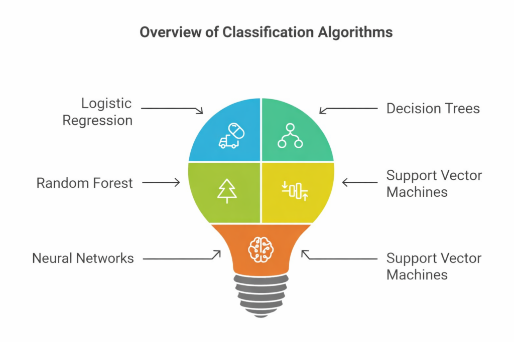
Popular Classification Algorithms In Machine Learning
Several algorithms can be used for classification tasks. Some of the most common and widely used ones include:
1. Logistic Regression
- Despite its name, logistic regression is used for classification, not regression.
- It is a simple and effective algorithm that predicts the probability of an instance belonging to a particular class.
- If the probability is above a certain threshold, the instance is assigned to one class, otherwise, it is assigned to another class.
Pros:
- Simple to implement and easy to understand.
- Works well for linearly separable data (where the classes can be separated by a straight line or a hyperplane).
Cons:
Not ideal for data with complex relationships, as it assumes a linear relationship between the features and the target.
2. Decision Trees
Decision trees are a popular classification algorithm. They work by recursively splitting the data based on the most important feature at each level, creating branches that lead to a decision (the class label).
Pros:
- Easy to understand and interpret.
- Can handle both numerical and categorical data.
Cons:
Can overfit if the tree is too deep (i.e., it memorizes the training data instead of learning general patterns).
3. Random Forest
Random Forest is an ensemble method that builds multiple decision trees and combines their predictions to improve accuracy.
By averaging the predictions from several trees, random forests can reduce the likelihood of overfitting compared to a single decision tree.
Pros:
- More accurate and robust than individual decision trees.
- Handles large datasets and complex data well.
Cons:
Slower to train and harder to interpret due to the complexity of the ensemble of trees.
4. Support Vector Machines (SVM)
SVM is a powerful algorithm that aims to find the best hyperplane that separates data into classes.
It tries to maximize the margin between the classes, which helps to improve the model’s ability to generalize.
SVM can also use kernels to map data into higher dimensions, enabling it to classify non-linearly separable data.
Pros:
- Effective for high-dimensional data (lots of features).
- Good at avoiding overfitting.
Cons:
Computationally expensive, especially for large datasets.
Requires careful parameter tuning to work optimally.
5. Neural Networks
Neural networks are inspired by the structure of the human brain and are particularly effective for handling complex problems like image recognition or natural language processing.
A neural network consists of layers of interconnected neurons, each processing the input data and passing the results to the next layer.
Pros:
- Can learn very complex patterns in data.
- Often produces state-of-the-art performance in fields like image recognition, speech processing, and natural language understanding.
Cons:
Requires large amounts of data and computational power.
The decision-making process of neural networks is often difficult to interpret (a “black box” problem).

Measuring Performance of Classification Models
Once you have trained a classification model, you need to evaluate its performance to see how well it works. Here are some common metrics used to evaluate classification models:
1. Accuracy
- Accuracy is one of the most straightforward and commonly used metrics.
- It measures the proportion of correct predictions made by the model out of all predictions. It is defined as:
\text{Accuracy} = \frac{\text{Number of Correct Predictions}}{\text{Total Number of Predictions}} = \frac{TP + TN}{TP + TN + FP + FN}
Where:
- TP = True Positives
- TN = True Negatives
- FP = False Positives
- FN = False Negatives
Limitation:
- While accuracy is easy to understand, it can be misleading, especially in imbalanced datasets.
- For example, in a dataset where 95% of the emails are not spam, a model predicting “not spam” for every email would have 95% accuracy but would fail to detect any spam.
2. Precision and Recall
Precision and recall are two metrics that provide more detailed insights into how well the model performs, especially when dealing with imbalanced classes.
Precision:
Precision measures the proportion of correctly predicted positive cases out of all predicted positives.
It answers the question:
“Out of all the instances predicted as positive, how many were actually positive?”
\text{Precision} = \frac{\text{True Positives}}{\text{True Positives + False Positives}} = \frac{TP}{TP + FP}
Interpretation: High precision means that when the model predicts a positive result, it is very likely to be correct.
Recall:
Recall, also known as sensitivity, measures the proportion of actual positive cases correctly identified by the model.
It answers the question:
“Out of all the actual positives, how many did the model catch?”
\text{Recall} = \frac{\text{True Positives}}{\text{True Positives + False Negatives}} = \frac{TP}{TP + FN}
Interpretation: High recall means the model is good at catching most of the positive instances, though it might also include some false positives.
3. F1 Score
- The F1 score combines both precision and recall into a single metric by calculating their harmonic mean.
- This is particularly useful when dealing with imbalanced datasets where a balance between precision and recall is important.
\text{F1 Score} = 2 \times \frac{\text{Precision} \times \text{Recall}}{\text{Precision} + \text{Recall}} = 2 \times \frac{TP}{2TP + FP + FN}
Interpretation: The F1 score gives a balance between precision and recall. A higher F1 score indicates a better model in terms of both detecting positives and avoiding false positives.
4. ROC Curve and AUC
ROC Curve (Receiver Operating Characteristic Curve):
- The ROC curve shows the trade-off between the true positive rate (TPR) and the false positive rate (FPR) at different classification thresholds.
- As the threshold is adjusted, the TPR and FPR change, and the ROC curve provides a way to visualize this trade-off.
- \text{True Positive Rate (TPR)} = \frac{\text{True Positives}}{\text{True Positives + False Negatives}} = \text{Recall}
- \text{False Positive Rate (FPR)} = \frac{\text{False Positives}}{\text{False Positives + True Negatives}}
AUC (Area Under the Curve):
- The AUC represents the area under the ROC curve. The value of AUC ranges from 0 to 1, where a value closer to 1 indicates a better-performing model.
- An AUC of 0.5 suggests that the model is no better than random guessing.
\text{AUC} = \text{Area Under the ROC Curve}
Interpretation: The ROC curve and AUC give insights into the model’s ability to discriminate between the positive and negative classes across different thresholds. A higher AUC value indicates better model performance.
Challenges in Classification
While classification is a powerful tool, there are several challenges that can affect its performance:
1. Imbalanced Data
- In many real-world problems, one class may have significantly more examples than the other.
- For example, in fraud detection, fraudulent transactions may be much fewer than legitimate transactions.
- This imbalance can lead to a model that is biased toward the majority class.
Solutions:
- Resampling: You can resample the dataset to either oversample the minority class or undersample the majority class.
- Specialized Algorithms: Some algorithms, like random forests or SVM, can handle imbalanced data better.
- Alternative Metrics: Use metrics like precision, recall, or F1 score instead of accuracy, as they provide a more nuanced view of performance.
2. Overfitting:
Overfitting occurs when the model learns the training data too well, including noise and outliers, which results in poor generalization to new data.
Solutions:
- Cross-validation: Cross-validation helps assess the model’s performance on unseen data and avoid overfitting.
- Regularization: Regularization techniques like L1 or L2 can be used to penalize overly complex models.
- Simpler Models: Sometimes simpler models, like logistic regression or decision trees, may perform better by preventing overfitting.
3. Feature Selection
Not all features are relevant for making predictions. Including irrelevant features can lead to overfitting or confusion in the model.
Solutions:
- Feature Importance: Some algorithms, like decision trees, can be used to assess the importance of each feature.
- Feature Selection Methods: Techniques like Recursive Feature Elimination (RFE) can help identify the most relevant features for the task.
Real-World Applications of Classification
Classification is used across various industries to solve important problems. Here are a few key applications:

Conclusion
Classification is a powerful machine learning task that helps us categorize data based on historical examples.
It has wide applications in fields like healthcare, finance, marketing, and natural language processing.
By understanding the core concepts, algorithms, and challenges of classification, you can apply this knowledge to solve real-world problems.
As machine learning continues to evolve, classification will play an even more significant role in driving innovation across many industries.
Frequently Asked Questions
Answer:
To become a data analyst, start by learning basic statistics, Excel, SQL, and a programming language like Python. After that, focus on data visualization and real-world projects. Building a strong portfolio and practicing with datasets can help you enter this field faster.
Answer:
A data analyst should know data cleaning, data visualization, basic mathematics, and problem-solving skills. Knowledge of tools like spreadsheets, databases, and visualization platforms is also important for career growth.
Answer:
Yes, a data analytics with AI course can be helpful for beginners because it combines traditional data analysis with modern AI concepts. It helps learners understand automation, predictive analysis, and smart data processing techniques.
Answer:
Such courses usually cover data analysis fundamentals, machine learning basics, data visualization, and AI-driven insights. You also learn how to interpret data to support business decisions.
Answer:
The learning time depends on your background. With consistent learning and practice, you can gain basic job-ready skills within 4–8 months. Advanced expertise may take longer depending on practice and project experience.
Answer:
Certifications can help demonstrate your knowledge and improve your resume. However, practical skills, projects, and problem-solving ability are often more important than certificates alone.
Answer:
Yes, many people enter data analytics from non-technical backgrounds. Starting with basic statistics, data handling, and beginner-friendly tools can make the transition easier.
Answer:
Classification is a machine learning technique used to categorize data into different groups based on patterns. It is commonly used in spam detection, fraud detection, and recommendation systems.
Answer:
The main types include binary classification (two categories), multi-class classification (more than two categories), and multi-label classification (multiple labels assigned to one input).
Answer:
Classification helps businesses and systems make predictions based on past data. It improves decision-making by automatically identifying patterns and grouping information correctly.